ManualFlowgaugeProcessor
1. What is a Sontek RS5 ADCP?
An Acoustic Doppler Current Profiler (ADCP) uses sound waves and the resulting Doppler shift to calculate flow-velocity.
The sensor is towed or driven over a cross-section of the water body emitting sound waves at a regular interval, each of these vertical 'ensembles' are stitched together to form a transect (cross-section).
Link to manufacturers webpage: (https://www.xylem.com/en-uk/products--services/analytical-instruments-and-equipment/flowmeters-velocimeters/rs5/)
2. Extracting Survey Data
It is expected that when exporting ADCP surveys off of the Sontek RS5, each survey is exported as a folder contaning the following files:
- 1x .rsqmb file (redundant for this package)
- 1x .dis file
- 1x .kml file
- 1x .sum file per transect
- 1x .ENU.vel file per transect
- 1x .snr file per transect
This is also the format that is expected from extract_sontekadcp_surveys.
Multiple unique survey files
If multiple .dis or .kml files are found in a folder, the first one will be used and a warning that multiple files have been found will be displayed
The following extract function creates a list of SontekADCPSurvey class objects with high-level metadata and specific sub-files as attributes.
from flowgaugeprocessor.extract import extract_sontekadcp_surveys

path = "path_to_your_SontekADCP_survey_folders"

surveys = extract_sontekadcp_surveys(path)
Transect Geo-Location Data
Try setting plot_transects=True to see all of the geo-tracking for each transect as they are extracted
3. Exporting Survey Data
If you simply want to export all of your survey data out into more standard file-formats, exporting single or grouped surveys will create either csv or parquet files contaning the data contained within the raw survey files.
Options for dataframe at the survey level:
"metadata": One row per survey. All survey metadata, location, datetime, equipment information; flow, depth and cross-section information"dis": One row per transect. All transect metadata, duration, quality-control; flow, depth and cross-section information
Options for dataframe at the transect level:
"sum": One row per ensemble. All ensemble metadata, ADCP sensor direction and velocity, angle and recorded depth for each of the four sensors"vel": One row per transect. All ensemble metadata, column per cell for each of the four sensors contaning flow velocity data"snr": One row per transect. All ensemble metadata, column per cell for each of the four sensors containing sensor dB data
3.1 Single Survey Export
Function to be added, creates all files mentioned above, 1x per survey.
3.2 Group Survey Export
For bulk exporting all extracted surveys in a single file, can be split back into individual surveys using the "site_id" and "site_name" columns.
3.2.1 Survey Level Export
from flowgaugeprocessor.extract import extract_sontekadcp_surveys
from flowgaugeprocessor.utils import export_group_survey_data

input_path = "path_to_your_SontekADCP_survey_folders"
output_path = "path_to_your_output_directory"

surveys = extract_sontekadcp_surveys(path)

export_group_survey_data(
    surveys=surveys,
    survey_type="SontekADCP",
    dataframe="metadata",
    export_path=out_path,
    file_out_name="ADCP Metadata",
    add_metadata=False,
    file_type="csv")

export_group_survey_data(
    surveys=surveys,
    survey_type="SontekADCP",
    dataframe="dis",
    export_path=out_path,
    file_out_name="ADCP Summary Data",
    add_metadata=False,
    file_type="csv")
3.2.2 Transect Level Export
from flowgaugeprocessor.extract import extract_sontekadcp_surveys
from flowgaugeprocessor.utils import export_group_transect_data

input_path = "path_to_your_SontekADCP_survey_folders"
output_path = "path_to_your_output_directory"

surveys = extract_sontekadcp_surveys(path)

export_group_transect_data(
    surveys=surveys,
    dataframe="sum",
    export_path=out_path,
    file_out_name="Transect Summary Data",
    file_type="csv")

export_group_transect_data(
    surveys=surveys,
    dataframe="vel",
    export_path=out_path,
    file_out_name="Transect Velocity Data",
    file_type="csv")

export_group_transect_data(
    surveys=surveys,
    dataframe="snr",
    export_path=out_path,
    file_out_name="Transect Sensor Data",
    file_type="csv")
3.3 Site Timeseries Export
Note: Function is a WIP as final format is being developed
To add: Option for file type, currently only parquet
For exporting a minimal timeseries file for each site surveted, contains:
"Discharge"- recorded in m³/s,"Mean-depth"- recorded in m,"Temperature"- not recorded by the RS5 ADCP,"Survey Type"- classified as"ADCP"for the RS5 ADCP
from flowgaugeprocessor.extract import extract_sontekadcp_surveys
from flowgaugeprocessor.fdri_timeseries_export import survey_to_fdri_timeseries

input_path = "path_to_your_SontekADCP_survey_folders"
output_path = "path_to_your_output_directory"

surveys = extract_sontekadcp_surveys(path)

surveys_to_fdri_timeseries(surveys, output_path)
Combine Your Equipment
This function works with multiple survey types, try joining all your survey lists together and applying the function
4. Plotting Survey Data
4.1 Transect Geo-Tracking
Transect geotracks can be plot using a Transect class method "plot_geodata()".
The three methods are:
- Bottom-Track: Compassed based tracking method, usually standard method chosen for final transect geotrack but can suffer from magnetic interference which can be seen in a characteristic curve or smiley face shape in the track (shown in the right-hand figure below). Uses a combination of relative position and Doppler shift so the errors will compound over the course of a transect.
- GGA: GPS based, calculates geotrack only using position of ADCP so can be more prone to errors on individual measure- ments but errors do not compound.
- Vtg: GPS based method, calculates position using the Doppler shift between the ADCP and the satellite. More accurate on individual location measurements but errors compound over the course of a transect.
The method used for each transect can be seen either as a Transect class attribute or in the summary output for a survey using either "export_single_survey_data()" or"export_group_survey_data()"
from flowgaugeprocessor.extract import extract_sontekadcp_surveys

input_path = "path_to_your_SontekADCP_survey_folders"

surveys = extract_sontekadcp_surveys(path)

surveys[2].transects[4].plot_geodata()
surveys[1].transects[3].plot_geodata()
4.2. Transect Cross-Sections
Transect cross-sections can be plot by referencing the survey and transect index in "surveys".
4.2.1 Transect Velocity Cross-Section
The standard plot_transect_cross_section(transect=transect) function creates the 'generic' cross-sectional plot showing the flow velocity recorded in each cell.
This automatically includes a small amount of pre-processing which can be toggled using an input-parameter, along with multiple other processing and plotting options.
from flowgaugeprocessor.extract import extract_sontekadcp_surveys
from flowgaugeprocessor.fdri_timeseries_export import plot_transect_cross_section

input_path = "path_to_your_SontekADCP_survey_folders"

surveys = extract_sontekadcp_surveys(path)

plot_transect_cross_section(surveys[0].transects[1])
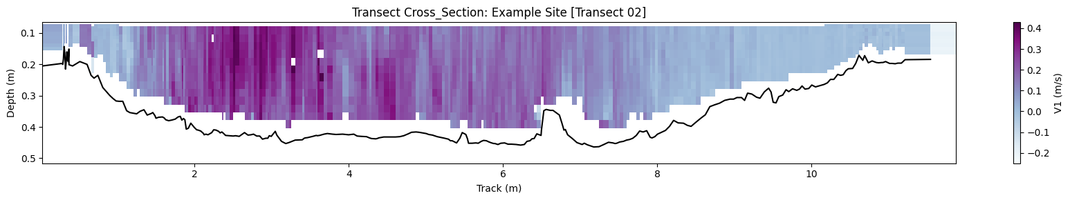
Add Profile Bar
Try setting show_beam_type=True to see which beam the sensor used to generate each vertical ensemble
Explore all the sensors
Try setting vX=V2 (or "V3", "V4") to see the velocity recorded by the other sensors, each sensor records the flow velocity in a different direction which are combined to calculate the final flow.
Note: "V1" has the largest component of downstream velocity.
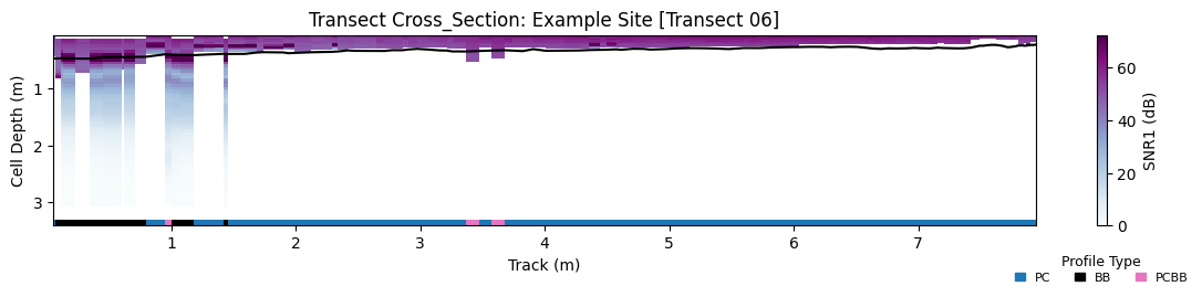
4.2.1 Transect Sensor Cross-Section
Plotting sensor information as a cross-section is less informative about the flow itself but can be utilised as a quality-control method and provides some interesting insight into the workings of the various beam-types used by the Sontek RS5.
from flowgaugeprocessor.extract import extract_sontekadcp_surveys
from flowgaugeprocessor.fdri_timeseries_export import plot_transect_sensor_cross_section

input_path = "path_to_your_SontekADCP_survey_folders"

surveys = extract_sontekadcp_surveys(path)

plot_transect_sensor_cross_section(surveys[1].transects[5])
Appendix 1: Equations Behind ADCP Data
Unlike acoustic flowsticks, the ADCP only records measurements from the surface. Thankfully, using Snell's law the flow velocity at layers below the surface can be calculated using only variables measured at the surface.
Snell’s Law
Where:
- \(\theta_{\alpha}\) is the angle of refraction
- \(\theta_{\beta}\) is the angle of incidence
- \(u\) is the speed of the wave in the medium
ADCP Doppler Shift
Where:
- \(D_{n}\) is the Doppler shift
- \(U_{n}\) is the horizontal component of river flow velocity
- \(F\) is the frequency of the transducer
- \(C_{n}\) is the speed of sound at the transducer
- \(\theta_{n}\) is the angle of the transducer to the vertical
- \(n\) is the layer being measured
The numerator is multiplied by 2 because the sound wave travels to the riverbed and then returns.
Snell’s Law Applied to ADCP
Given two measurements at different depths with velocities \(U_{1}\) and \(U_{2}\), speeds of sound \(C_{1}\) and \(C_{2}\), and angles \(\theta_{1}\) and \(\theta_{2}\), the Doppler shifts \(D_{1}\) and \(D_{2}\) are:
Using Snell’s Law:
This implies:
Therefore:
The term \(-2 F \sin(\theta_{1}) C_{1}\) cancels out, showing that the change in Doppler shift depends only on \(U\).
Consequently, the velocities can be calculated using only the known transducer frequency \(F\), the recorded Doppler shift \(D_{n}\), the speed of sound in the first layer \(C_{1}\), and the transducer angle \(\theta_{1}\):